usensys

A minimal example

The package currently includes a reduced version of a 26-zone model developed for Model Intercomparison Project. Data for the original model will be published in separate repository. The simplified version has lower granularity but the same structure.

library(tidyverse)
library(usensys)
# set_scenarios_path()
get_scenarios_path() # get the path to the scenarios
#> [1] "scenarios/"
set_default_solver(solver_options$julia_highs_barrier) # for small-scale models
# CPLEX or Gurobi are recommended for large models
# set_default_solver(solver_options$julia_cplex_barrier) 
set_progress_bar() # shoe progress bar for the long operations

Also make sure that Julia, Python, or GAMS are installed and the paths are set.

26-zone model

names(usensys::us26min) # the model elements with data
names(usensys::calendars) # alternative calendars for the model
names(usensys::horizons) # alternative horizons for the model

The list us26min contains repositories with different model elements. A complete model should have the following elements:

• declaration of commodities
  
• declaration of primary supply
  
• declaration of the final demand
  
• declaration of the technological processes such as generators, storage
  

Optional elements are:

• declaration of interregional trade, such as transmission lines
  
• declaration of international trade
  
• declaration of ‘weather’ factors for variable resources
  
• policy and other constraints, such as CO2 cap, capacity and retirement constraints, etc.
  

Data

The data for the model including all technologies, capacity factors, commodities, supply and demand is stored in the respective classes of energyRt, grouped in different repositories, and stored in the package data. Here we use the us26min repository that contains the data for the 26-zone model. The following step shapes the model structure by combining the model elements into a single repository.

# Combine model elements that are used in all scenarios in a "main" repository
attach(us26min) # attach the model elements to the environment 
repo_main <- newRepository(
  name = "repo_main",
  desc = "US 26-zone minimal model for testing",
  repo_comm, # commodities
  repo_sup, # primary supply
  repo_storage, # storage with weekly cycle
  # repo_storage_fy, # storage with full-year cycle
  repo_chargelinks, # charging and discharging capacity optimization for storage
  repo_chargelinks_cn, # sets charging capacity equal to discharging capacity
  repo_weather, # capacity factors for wind, solar, and hydro
  repo_vre, # variable renewable energy sources: wind, solar, hydro
  repo_nuclear, # nuclear generators
  repo_hydroelectric, # hydroelectric generators
  repo_geothermal, # geothermal generators
  # thermal
  repo_coal, # coal generators
  repo_naturalgas, # natural gas generators
  repo_other, # other generators
  repo_biomass, # biomass generators
  repo_hydrogen, # hydrogen technologies
  # trade
  repo_trade, # interregional transmission lines
  # CO2CAP_US, # National CO2 cap 
  LOSTLOAD, # Lost load penalty
  DEMELC # Load projections by zone and hour  
  ) 
detach(us26min) # detach the model elements
summary(repo_main)

Other model elements/objects can be added or replaced later to specify scenarios.

Model

Objects in the repo_main repository are used in all scenarios and stored in the created on the next step model object.

# Declaration of the model
mod <- newModel(
  name = "US26min", # name of the model
  desc = "US 26-zone minimal model for testing", # description
  # Default configuration
  region = usensys_maps$us26_sf$region, # names of all regions used in the model
  discount = .02, # discount rate
  calendar = calendars$calendar_52w, # full calendar with 52 weeks 
  horizon = horizons$horizon_2027_2050_by5, # default model horizon 
  optimizeRetirement = FALSE, # optimization of the retirement is disabled
  # Data: add model elements used in all scenarios
  data = repo_main
)
rm(repo_main) # clean up

Interpolation and solving the model

The model can be solved in one or four steps. solve function applied to the model object will complete all four steps. For large models it is recommended to split the process into four steps to monitor the progress and avoid the repetition of time-consuming steps such as the interpolation and solution.

The time required to solve the model can vary widely. Beyond hardware factors (such as processor speed, number of cores, and RAM size and speed), the solver and algorithm choice play crucial roles. At the time of writing this vignette, there is a significant performance gap between commercial and open-source solvers. Commercial solvers are capable of solving the full model, including all hours and multi-year optimizations. Open-source solvers can be used to solve the model with sampled time-slices in a reasonable time frame.

Solving scenarios

The example below demonstrates the process of solving the model in four steps for two scenarios. Reference (REF) scenario assumes no policy intervention, while the Carbon Cap (CAP) scenario includes a CO2 cap. For a testing purpose, the model is solved for a subset of just a few time-slices but full horizon. Such sampled model can be solved using open-source solvers HiGHS, CBC, or GLPK.

1. Interpolation of the model/scenario parameters

scen_REF_test <- interpolate(
  mod, # model object
  name = "REF_test", # name of the scenario
  desc = "Test REF scenario on 4-days 6-hours data", # description
  calendar = calendars$calendar_4d_6h # replace default calendar
)
summary(scen_REF_test)

scen_CAP_test <- interpolate(
  mod, # model object
  name = "CAP_test", # name of the scenario
  desc = "Test CAP scenario on 4-days 6-hours data", # description
  us26min$CO2CAP_US, # add CO2 cap
  calendar = calendars$calendar_4d_6h # subset calendar
)

2. Writing the model script and scenario data

scen_REF_test <- write_sc(
  scen_REF_test, # interpolated scenario
  solver = solver_options$julia_highs_barrier # (optional) replaces the default solver
) 
scen_CAP_test <- write_sc(
  scen_CAP_test,
  solver = solver_options$julia_highs_barrier # replace the default solver
)

3. Solving the model/scenario

scen_REF_test <- solve_scenario(scen_REF_test, wait = TRUE) 
scen_CAP_test <- solve_scenario(scen_CAP_test, wait = TRUE) 
# use wait = FALSE to run scenarios in parallel

4. Reading the results

scen_REF_test <- read(scen_REF_test)
scen_CAP_test <- read(scen_CAP_test)

summary(scen_REF_test)
summary(scen_CAP_test)

Quick look at the results

# Store solved scenarios in a list
sns <- list(scen_REF_test, scen_CAP_test)

# Objective values
getData(sns, "vObjective", merge = TRUE)
#> # A tibble: 2 × 3
#>   scenario name         value
#>   <chr>    <chr>        <dbl>
#> 1 REF_test vObjective 8.68e11
#> 2 CAP_test vObjective 1.20e12

## New capacity
getData(sns, "vTechNewCap", merge = TRUE, digits = 1, process = T) %>%
  # filter out charger capacity (equal to the dis-chargers)
  filter(!grepl("_discharger", process)) %>%
  # remove cluster and group identifiers from the process names
  # (this process will be automated in the future versions of the package)
  mutate(process = gsub("_(C|CL|FG)[0-9]+", "", process)) |>
  # remove "charger" from the process names
  mutate(process = gsub("_charger", "", process)) |>
  mutate(process = gsub("_(C|CL|FG)[0-9]+", "", process)) |>
  group_by(scenario, process, year) %>%
  summarise(GW = sum(value)/1e3, .groups = "drop") |>
  ggplot() +
  geom_bar(aes(x = as.factor(year), y = GW, fill = process), 
           stat = "identity") +
  facet_grid(. ~ scenario) +
  scale_fill_viridis_d(option = "H") +
  labs(x = "") +
  theme_bw()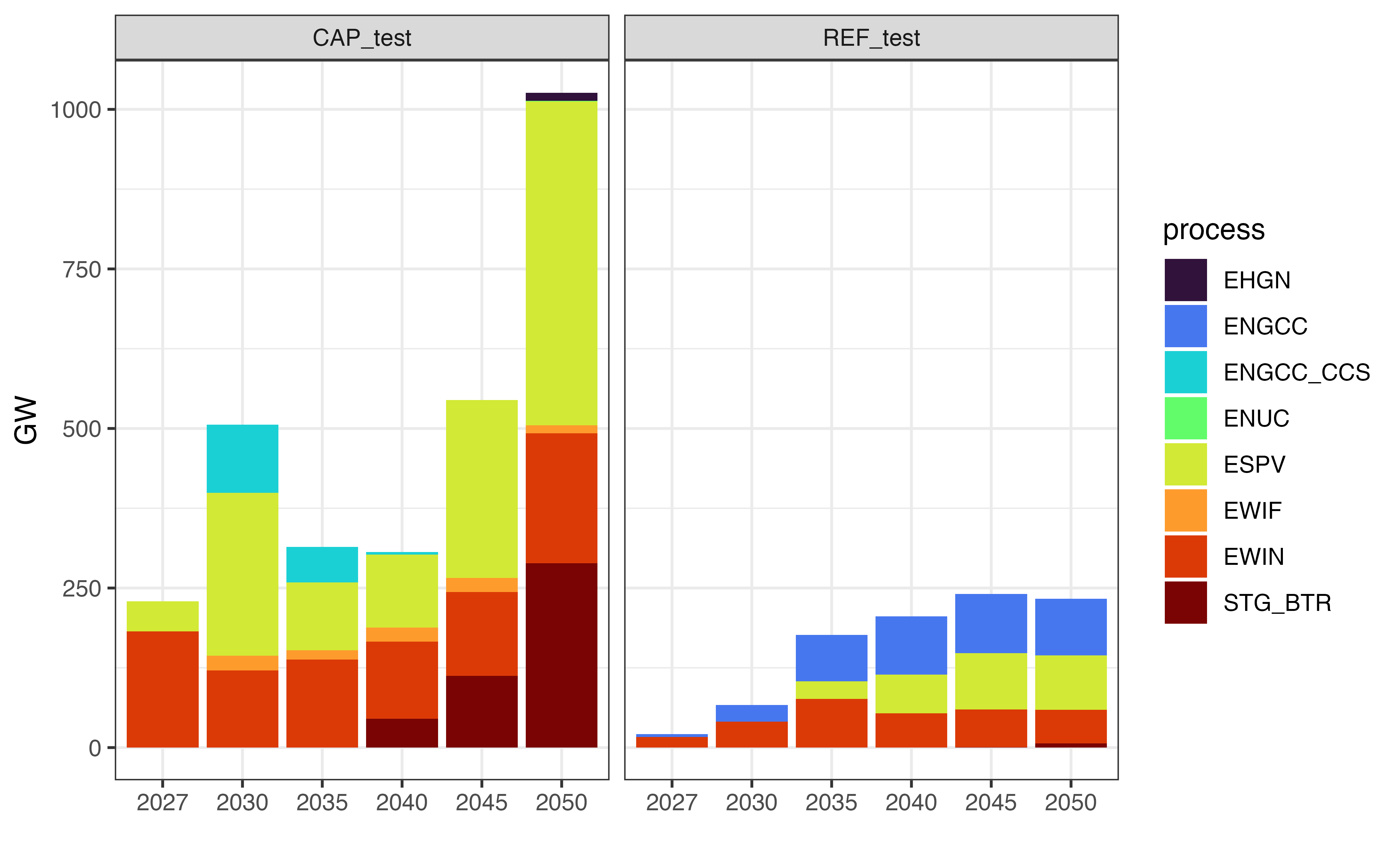

New capacity, GW

# Carbon emissions
getData(sns, "vBalance", comm = "CO2", merge = TRUE) %>%
  group_by(scenario, year) %>%
  summarise(GtCO2 = sum(value)/1e6, .groups = "drop") |>
  ggplot() +
  geom_line(aes(x = year, y = GtCO2, color = scenario), linewidth = 1.5) +
  geom_point(aes(x = year, y = GtCO2, color = scenario), size = 3) +
  # scale_fill_viridis_d(option = "H") +
  labs(x = "") +
  theme_bw()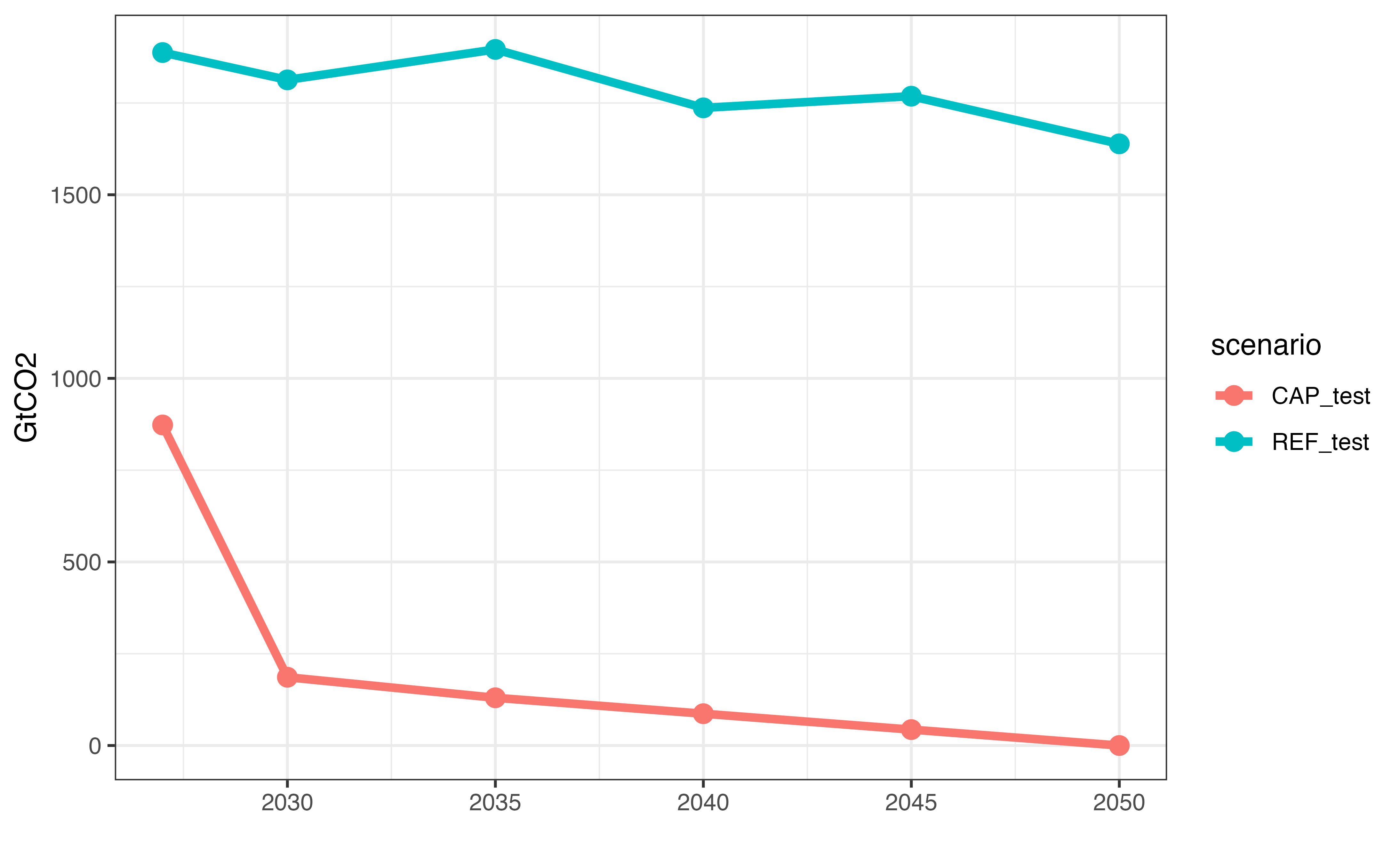

Carbon emissions, GtCO2

The full list of variables and parameters is available in the energyRt documentation which is in the progress.

Scenario objects contain all the data about the model and the solution, including the model script, raw and interpolated inputs, and the results. See slotNames(scen_REF_test) and help('scenario-class') for more details.

Scenarios can be saved and loaded using the standard R functions save and load.

# Save scenarios
save(scen_REF_test, file = file.path(scen_REF_test@path, "scen_REF_test.RData"))
save(scen_CAP_test, file = file.path(scen_CAP_test@path, "scen_CAP_test.RData"))

For scenarios with large data, it is recommended to save them in an arrow-parquet format using the save_scenario() function. By default it will save the scenario in the get_scenarios_path() directory along with the model script and the results.

scen_REF_test@path
save_scenario(scen_REF_test)

scen_CAP_test@path
save_scenario(scen_CAP_test)

Loading saved scenarios can be done using the load_scenario() function pointing it to the directory with the saved scenario. The function returns a scenario object in a separate .scen environment. However instead of data, slots contain references to the data stored on disk.

load_scenario("scenarios/REF_test_US26min_4d_6h_Y2027_2050_by5")
load_scenario("scenarios/CAP_test_US26min_4d_6h_Y2027_2050_by5")
ls(.scen)
sns <- list(.scen$scen_REF_test, .scen$scen_CAP_test)

The data can be accessed with the same functions as for the original scenario object

getData(sns, "vTradeNewCap", merge = TRUE, digits = 0) |>
  group_by(scenario, trade) |>
  summarise(GW = sum(value)/1e3, .groups = "drop") |>
  pivot_wider(names_from = scenario, values_from = GW) |>
  arrange(desc(CAP_test + REF_test)) |>
  head(10) |>
  kableExtra::kable(caption = "Table. Transmission, new capacity, GW") |>
  kableExtra::kable_styling(bootstrap_options = "striped", full_width = T)

Table. Transmission, new capacity, GW

trade	CAP_test	REF_test
PJMD_to_PJME	29.769	0.070
MISS_to_SPPS	20.372	3.916
ISNE_to_NYUP	24.174	0.000
NYUP_to_PJME	18.047	0.000
PJME_to_PJMW	16.465	0.000
MISS_to_SPPC	13.407	0.000
SRCA_to_SRSE	12.199	0.000
SPPC_to_SPPN	4.667	7.086
PJMC_to_PJMW	10.632	0.000
PJMD_to_SRCA	10.402	0.000

While a sampled model does not fully capture the variability in load and weather-driven capacity factors of renewable energy sources, it is useful for testing purposes. It allows for comparing the performance of different solvers, as well as experimenting with various time-slice configurations. This approach offers a fast way to test models or scenarios on consumer-grade desktops or laptops before performing large-scale optimizations on high-performance workstations or in the cloud.

The choice of time-slices (weeks, hours) to be included or omitted in a scenario is arbitrary in this example. There are several alternative subset calendars available in the package (data(calendars)) with alternative selections of time-slices (names(calendars)):

• calendar_52w is the full calendar of the model with 52 weeks and 168 hours per week, 8736 hours per year in total
• calendar_4w - subset of 4 weeks, 168 hours per week, 672 hours per year in total
• calendar_12d - 12 days, 24 hours per day where every day is from a different month, 288 hours per year in total
• calendar_4d_6h - a reduced version of calendar_4w with 4 days and 6 hours per day, 24 hours per year in total.

Calendars with custom selections of time-slices can be created using the subset_calendar() function.

Solving 52-week model

tbc…